Example: Visium Human DLPFC
Source:vignettes/example_visium_human_DLPFC.Rmd
example_visium_human_DLPFC.RmdApplication of Spacelink to Visium Human DLPFC Dataset
This vignette demonstrates how to perform spatial gene expression
analysis using the spacelink package with Visium human
dorsolateral prefrontal cortex (DLPFC) dataset. The dataset is available
here, where we used
sample 151673. Cell-type proportions were estimated using RCTD with the CosMx
Human Frontal Cortex dataset as the reference. The processed example
data, saved as Visium_human_DLPFC, includes gene
expression, spot coordinates, and the estimated cell type
proportions.
Load example dataset
data(Visium_human_DLPFC)
counts <- Visium_human_DLPFC$counts
spatial_coords <- Visium_human_DLPFC$spatial_coords
dim(counts)
## [1] 33538 3639
dim(spatial_coords)
## [1] 3639 2Preprocessing
# Filter mitochondrial and low-expressed genes
counts <- counts[!grepl("(^MT-)|(^mt-)", rownames(counts)),]
counts <- counts[rowSums(counts >= 3) >= ncol(counts)*0.005,]
dim(counts)
## [1] 3309 3639
# Normalize expression counts using sctransform package
seurat_obj <- CreateSeuratObject(counts = counts)
seurat_norm = SCTransform(seurat_obj, vst.flavor = "v2", verbose = FALSE)
normalized_counts <- seurat_norm@assays$SCT$data
Run global Spacelink
# Here, we investigate eight example genes.
gene_list = c("CNP","SHISA5","PHB","HOPX","MOBP","EIF5B","SCGB2A2","YWHAE")
global_results <- spacelink_global(normalized_counts = normalized_counts[gene_list,],
                                   spatial_coords = spatial_coords)
print(global_results)
##            tau.sq  sigma.sq1    sigma.sq2    sigma.sq3    sigma.sq4 sigma.sq5        phi1         phi2         phi3         phi4         phi5     raw_ESV  time       pval1       pval2         pval3         pval4         pval5        pval        padj         ESV
## CNP     0.0000000 0.00000000 0.7015934749 0.2179618252 0.000000e+00         0 0.001048406 0.0009286621 0.0008225946 0.0007286417 0.0006454196 0.994768081 4.999 0.000000000 0.000000000  0.000000e+00  0.000000e+00  0.000000e+00 0.000000000 0.000000000 0.994768081
## SHISA5  0.1500294 0.00000000 0.0004149912 0.0006837337 0.000000e+00         0 0.001703009 0.0013362057 0.0010484062 0.0008225946 0.0006454196 0.007209596 4.631 0.018972197 0.014445518  1.518510e-02  2.165076e-02  3.749959e-02 0.019186192 0.025581589 0.007209596
## PHB     0.1369763 0.00508862 0.0000000000 0.0000000000 0.000000e+00         0 0.007299270 0.0064655812 0.0057271124 0.0050729880 0.0044935748 0.026105641 4.189 0.118799139 0.110644681  1.091531e-01  1.136193e-01  1.235950e-01 0.114928890 0.131347303 0.000000000
## HOPX    0.1844922 0.00000000 0.0720213108 0.0766421489 2.561652e-03         0 0.001048406 0.0009286621 0.0008225946 0.0007286417 0.0006454196 0.448242916 4.147 0.000000000 0.000000000 2.611455e-312 5.377138e-281 2.750916e-250 0.000000000 0.000000000 0.448242916
## MOBP    0.0000000 0.00000000 0.4831314048 0.1345105327 0.000000e+00         0 0.001048406 0.0009286621 0.0008225946 0.0007286417 0.0006454196 0.994747311 4.422 0.000000000 0.000000000  0.000000e+00  0.000000e+00  0.000000e+00 0.000000000 0.000000000 0.994747311
## EIF5B   0.1113762 0.00000000 0.0000000000 0.0016466986 0.000000e+00         0 0.002766333 0.0021705050 0.0017030094 0.0013362057 0.0010484062 0.014321150 4.074 0.003477314 0.001992989  1.645165e-03  2.147440e-03  4.220251e-03 0.002381182 0.003809891 0.014321150
## SCGB2A2 0.0000000 0.13916786 0.7402986887 0.1394122051 0.000000e+00         0 0.001048406 0.0009286621 0.0008225946 0.0007286417 0.0006454196 0.994473609 4.939 0.000000000 0.000000000  0.000000e+00  0.000000e+00  0.000000e+00 0.000000000 0.000000000 0.994473609
## YWHAE   0.2485001 0.00000000 0.0011635764 0.0012691117 9.102338e-05         0 0.004493575 0.0039803394 0.0035257234 0.0031230316 0.0027663334 0.009273184 4.009 0.183838106 0.173973851  1.681146e-01  1.660988e-01  1.675962e-01 0.171708675 0.171708675 0.000000000
Investigate global Spacelink result
The primary results are as follows:
-
pval: Combined p-value for spatial significance -
padj: Benjamini-Hochberg adjusted p-values -
ESV: Effective Spatial Variability score (0-1)
# Number of significant SVGs
table(global_results$padj <= 0.05)
## FALSE TRUE
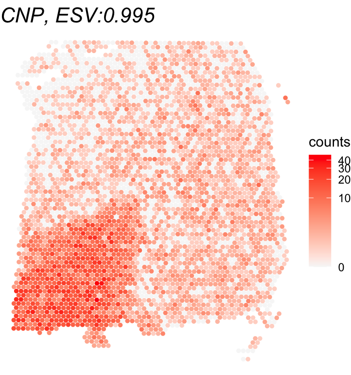
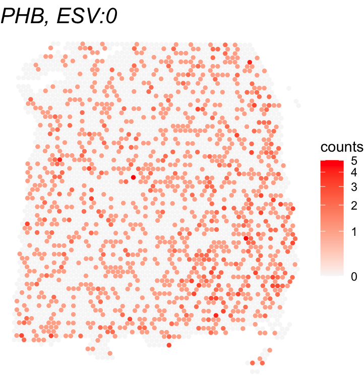
## 2 6Top-ranked SVGs can be identified using the ESV score. Shown here is an example plotting the SVG with the highest ESV and a non-SVG with the lowest ESV score.
# Plot of the top SVG (highest ESV) and a non-SVG (lowest ESV)
gene_names = rownames(global_results)[c(which.max(global_results$ESV),
                                        which.min(global_results$ESV))]
print(gene_names)
## [1] "CNP" "PHB"
for(gene_name in gene_names){
  df <- as.data.frame(cbind(spatial_coords, expr = counts[gene_name,]))
  colnames(df) <- c('X0', 'X1', 'expr')
  title <- paste0(gene_name, ", ESV:", round(global_results[gene_name,'ESV'],3))
  print(ggplot(df, aes(x = X0, y = X1, color = expr)) +
    geom_point(size = 1) +
    ggtitle(title) + theme_void() + scale_y_reverse() +
    scale_color_gradient(low = "grey97", high = "red", trans = "log1p", name = "counts") +
    theme(plot.title = element_text(face = "italic", size = 16)))
}
Run cell-type-specific Spacelink
# Load cell type proportions
cell_type_proportions <- Visium_human_DLPFC$cell_type_proportions
dim(cell_type_proportions)
## [1] 3639 9
colnames(cell_type_proportions)
## [1] "endothelial"  "L2_3"  "L4"  "L6"  "oligodendrocyte"
## [6] "OPC"  "astro"  "Inh"  "microglia"
# In this example, we examine the oligodendrocyte-specific spatial variability.
cell_type_results <-
  spacelink_cell_type(normalized_counts = normalized_counts[gene_list,],
                      spatial_coords = spatial_coords,
                      cell_type_proportions = cell_type_proportions,
                      focal_cell_type = "oligodendrocyte",
                      global_spacelink_results = global_results,
                      # The above is not required, though providing global results can improve efficiency.
                      calculate_ESV = TRUE)
print(cell_type_results)
##            time         pval          ESV
## CNP      89.171 2.198766e-11 6.739803e-01
## SHISA5   98.919 6.202876e-01 1.447781e-02
## PHB     119.905 3.490079e-01 3.660781e-02
## HOPX     83.524 7.563056e-01 1.991051e-05
## MOBP    135.633 4.283413e-02 6.835911e-01
## EIF5B   104.500 4.050604e-01 1.065050e-01
## SCGB2A2  86.259 1.338166e-08 9.615069e-01
## YWHAE    84.141 8.624388e-01 1.844341e-05
Investigate cell-type-specific Spacelink result
The key results are as follows:
-
pval: Combined p-value for spatial significance -
ESV: Cell-type-specific Effective Spatial Variability (ct-ESV) score (0-1)
# Number of significant ct-SVGs within oligodendrocyte
table(cell_type_results$pval <= 0.05)
## FALSE TRUE
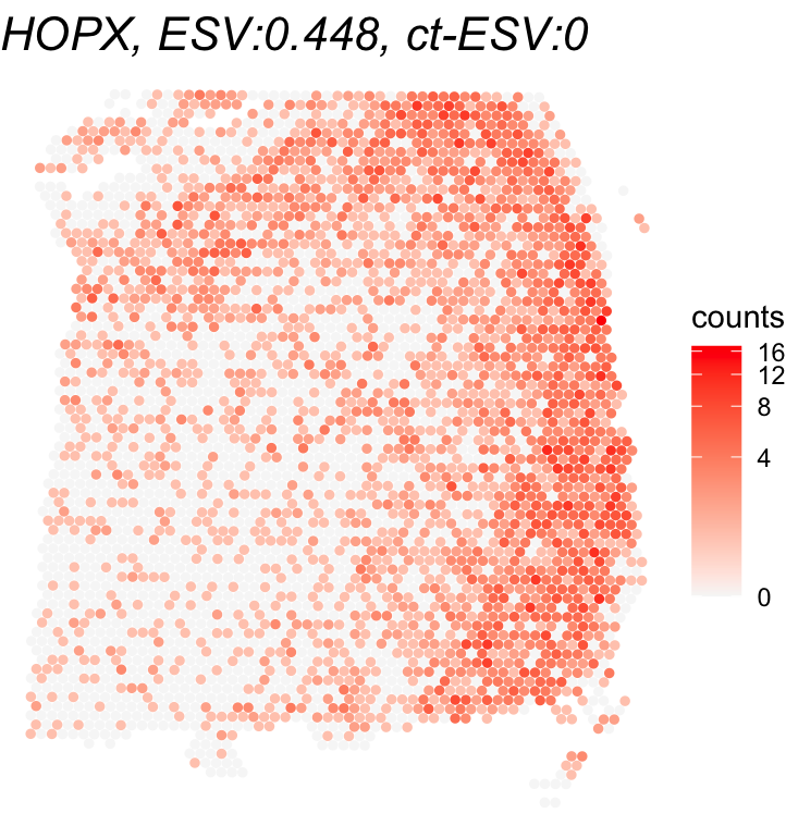
## 5 3 The following illustrates the ct-SVG with the highest ct-ESV and a non-ct-SVG with the lowest ct-ESV among significant global SVGs identified by the global Spacelink analysis.
# Plot of the top ct-SVG (highest ct-ESV) and a non-ct-SVG (lowest ct-ESV) among significant global SVGs
global_svg_names = rownames(global_results)[global_results$padj <= 0.05]
gene_names = global_svg_names[c(which.max(cell_type_results[global_svg_names,'ESV']),
                                which.min(cell_type_results[global_svg_names,'ESV']))]
print(gene_names)
## [1] "SCGB2A2" "HOPX"
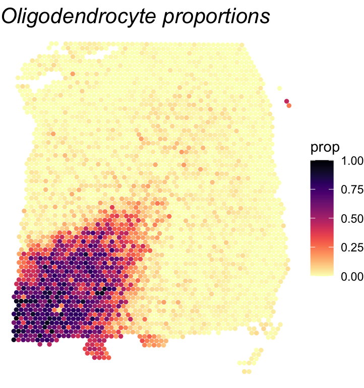
# Plot oligodendrocyte cell type proportions
df <- as.data.frame(cbind(spatial_coords, expr = cell_type_proportions[,'oligodendrocyte']))
colnames(df) <- c('X0', 'X1', 'prop')
print(ggplot(df, aes(x = X0, y = X1, color = prop)) +
        geom_point(size = 1) +
        ggtitle("Oligodendrocyte proportions") + theme_void() + scale_y_reverse() +
        scale_color_viridis(option="magma",direction=-1,limits=c(0,1)) +
        theme(plot.title = element_text(face = "italic", size = 16)))

# Plot gene expressions
for(gene_name in gene_names){
  df <- as.data.frame(cbind(spatial_coords, expr = counts[gene_name,]))
  colnames(df) <- c('X0', 'X1', 'expr')
  title <- paste0(gene_name, ", ESV:", round(global_results[gene_name,'ESV'],3),
                  ", ct-ESV:", round(cell_type_results[gene_name,'ESV'],3))
  print(ggplot(df, aes(x = X0, y = X1, color = expr)) +
          geom_point(size = 1) +
          ggtitle(title) + theme_void() + scale_y_reverse() +
          scale_color_gradient(low = "grey97", high = "red", trans = "log1p", name = "counts") +
          theme(plot.title = element_text(face = "italic", size = 16)))
}