Application of Spacelink to Visium Human DLPFC Samples across AD Progression Stages
In this vignette, we apply Spacelink to Visium brain dorsolateral prefrontal cortex (DLPFC) samples from donors at different stages of Alzheimer’s Disease (AD) to demonstrate that Spacelink can capture differences in spatial gene expression patterns associated with AD pathological features.
We use a dataset of 32 ROSMAP 10x Visium samples, available at link.
Here, we analyze PKM expression in one control sample and one late-stage AD sample. PKM is a key glycolytic enzyme that may be affected by metabolic dysfunction in early AD. We show that PKM exhibits distinct spatial expression patterns across AD stages, and that these differences can be captured by examining spatial variability using Spacelink.
2. Load Example Dataset
We use one control sample (ID: 50500136_1) and one late-stage AD sample (ID: 18414513_1).
control_spe <- readRDS("50500136_1.rds")
control_counts <- as.matrix(counts(control_spe))
control_spatial_coords <- as.data.frame(spatialCoords(control_spe))

AD_spe <- readRDS("18414513_1.rds")
AD_counts <- as.matrix(counts(AD_spe))
AD_spatial_coords <- as.data.frame(spatialCoords(AD_spe))

dim(control_counts)
## [1] 36601 1663
dim(AD_counts)
## [1] 36601 12733. Preprocessing
Before running the analysis, we remove mitochondrial genes and genes that are expressed in very few spots (less than 0.5%). Also, we normalize the counts using SCTransform.
control_counts <- control_counts[!grepl("(^MT-)|(^mt-)", rownames(control_counts)),]
control_counts <- control_counts[apply(control_counts >= 3, 1, sum) >= ncol(control_counts)*0.005,]
seurat_obj <- CreateSeuratObject(counts = control_counts)
seurat_norm = SCTransform(seurat_obj, vst.flavor = "v2", verbose = FALSE)
control_normalized_counts <- seurat_norm@assays$SCT$data

AD_counts <- AD_counts[!grepl("(^MT-)|(^mt-)", rownames(AD_counts)),]
AD_counts <- AD_counts[apply(AD_counts >= 3, 1, sum) >= ncol(AD_counts)*0.005,]
seurat_obj <- CreateSeuratObject(counts = AD_counts)
seurat_norm = SCTransform(seurat_obj, vst.flavor = "v2", verbose = FALSE)
AD_normalized_counts <- seurat_norm@assays$SCT$data

dim(control_normalized_counts)
## [1] 6825 1663
dim(AD_normalized_counts)
## [1] 4228 12734. Run Global Spacelink
We compute the Effective Spatial Variability (ESV) score for the PKM gene in each sample. A higher ESV indicates stronger spatial patterning of expression across tissue spots.
5. Visualize Results
We visualize three aspects of each sample side by side:
- Expression: raw PKM expression level
- Layer: cortical layer annotation per spot
- Plaque: proximity to neuritic plaques
colnames(control_spatial_coords) = c("x","y")
control_spatial_coords$expression = control_counts['ENSG00000067225',]
control_spatial_coords$layer = control_spe$SpatialCluster
control_spatial_coords$distance = control_spe$MinDistNP
control_spatial_coords <- control_spatial_coords %>%
  mutate(distance_category = case_when(
    distance <= 150 ~ "near",
    distance > 150  ~ "far",
    TRUE            ~ NA_character_
  ))

colnames(AD_spatial_coords) = c("x","y")
AD_spatial_coords$expression = AD_counts['ENSG00000067225',]
AD_spatial_coords$layer = AD_spe$SpatialCluster
AD_spatial_coords$distance = AD_spe$MinDistNP
AD_spatial_coords <- AD_spatial_coords %>%
  mutate(distance_category = case_when(
    distance <= 150 ~ "near",
    distance > 150  ~ "far",
    TRUE            ~ NA_character_
  ))

plot_gene = function(spatial_coords, ESV, dot_size = 1) {
  p1 <- ggplot(spatial_coords, aes(x = x, y = y, color = expression)) +
    geom_point(size = dot_size) +
    scale_color_viridis(option = "magma", direction = -1) +
    coord_fixed() +
    theme_minimal(base_size = 20) +
    theme(
      panel.grid     = element_blank(),
      axis.title     = element_blank(),
      axis.text      = element_blank(),
      axis.ticks     = element_blank(),
      plot.title     = element_text(face = "bold", hjust = 0.5)
    ) +
    labs(
      color = "Expression",
      title = paste0("Gene: PKM   ESV: ", ESV)
    )

  my_colors <- c(
    "#1f77b4", "#ff7f0e", "#2ca02c", "#d62728",
    "#9467bd", "#8c564b", "#e377c2", "#7f7f7f",
    "#bcbd22", "#17becf", "#a65628", "#f781bf"
  )
  p2 <- ggplot(spatial_coords, aes(x = x, y = y, color = layer)) +
    geom_point(size = dot_size) +
    coord_fixed() +
    scale_color_manual(values = my_colors) +
    theme_minimal(base_size = 20) +
    theme(
      panel.grid     = element_blank(),
      axis.title     = element_blank(),
      axis.text      = element_blank(),
      axis.ticks     = element_blank(),
      plot.title     = element_text(face = "bold", hjust = 0.5)
    ) +
    labs(
      color = "Layer",
      title = "Layer"
    )

  p3 <- ggplot(spatial_coords, aes(x = x, y = y, color = distance_category)) +
    geom_point(size = dot_size) +
    coord_fixed() +
    scale_color_manual(
      values = c("near" = "brown", "far" = "#dbd1c1"),
      labels = c("near" = "Plaque", "far"  = "Non-Plaque")
    ) +
    theme_minimal(base_size = 20) +
    theme(
      panel.grid     = element_blank(),
      axis.title     = element_blank(),
      axis.text      = element_blank(),
      axis.ticks     = element_blank(),
      legend.key.size= unit(0.8, "cm"),
      plot.title     = element_text(face = "bold", hjust = 0.5)
    ) +
    labs(color = "Distance", title = "Neuritic Plaque")

  return(list(expression = p1, layer = p2, plaque = p3))
}

control_plot = plot_gene(control_spatial_coords, round(control_ESV,4), dot_size = 2.3)
control_plot = control_plot[[1]] + guides(color="none") + control_plot[[2]] + guides(color="none") + control_plot[[3]] + guides(color="none")

AD_plot = plot_gene(AD_spatial_coords, round(AD_ESV,4), dot_size = 2.3)
AD_plot = AD_plot[[1]] + guides(color="none") + AD_plot[[2]] + guides(color="none") + AD_plot[[3]] + guides(color="none")

print(control_plot)
print(AD_plot)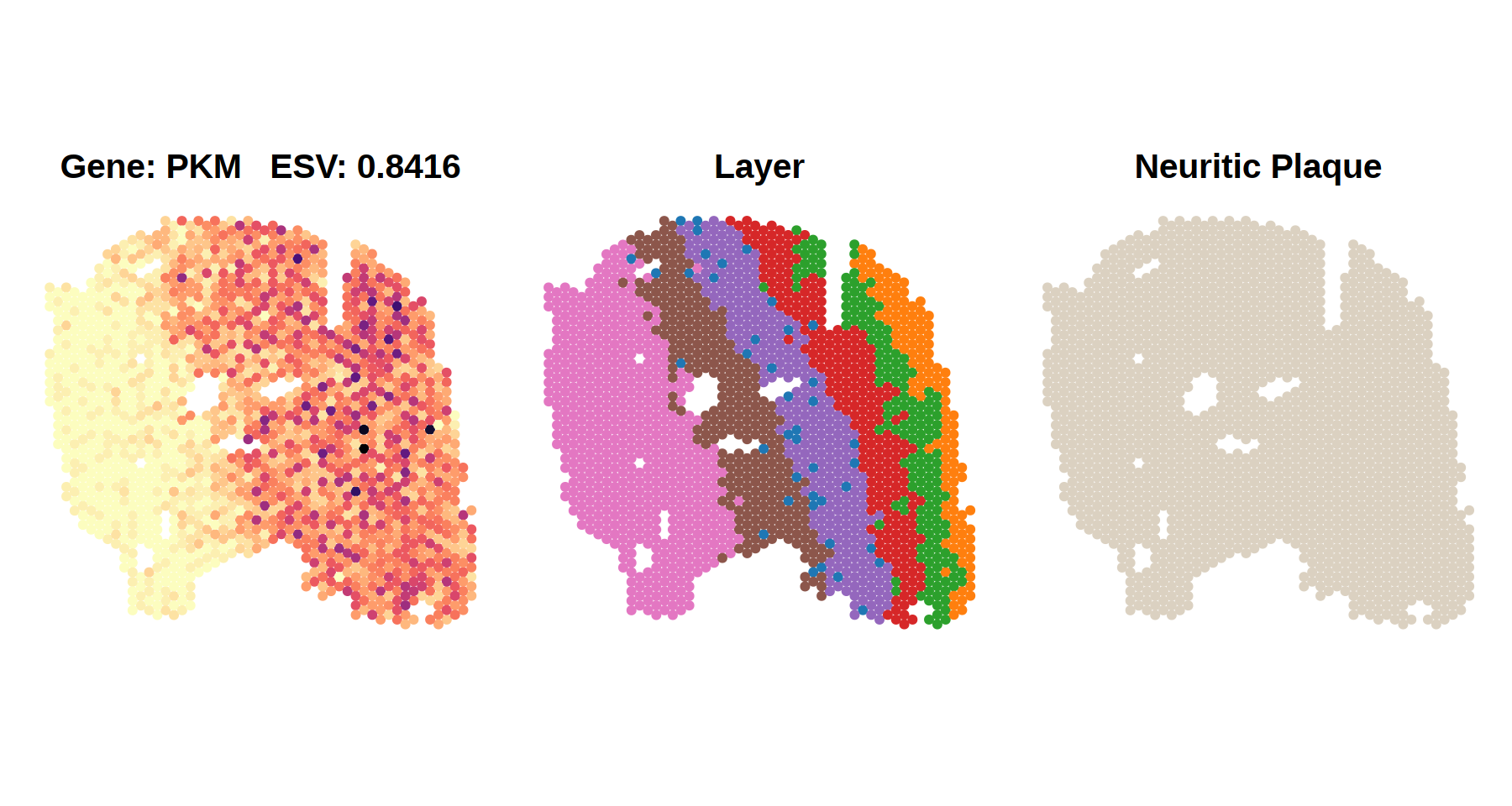
 In the control sample (top panel),
where no neuritic plaques are present, PKM expression aligns
with cortical layers, showing strong spatial patterning. This pattern is
captured by a high ESV score (0.8416).
In the control sample (top panel),
where no neuritic plaques are present, PKM expression aligns
with cortical layers, showing strong spatial patterning. This pattern is
captured by a high ESV score (0.8416).
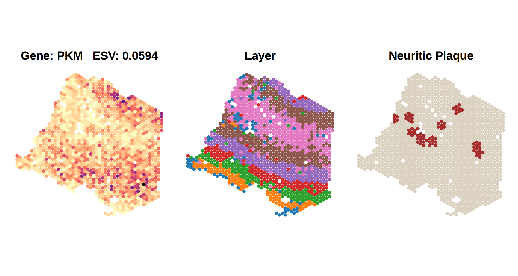
In contrast, in the late-stage AD sample (bottom panel), where multiple neuritic plaques are present, PKM expression appears disorganized and shows much weaker spatial patterning, reflected in a low ESV score (0.0594).
Together, these results demonstrate that Spacelink effectively captures AD-associated changes in spatial gene expression.