CosMx Human Frontal Cortex Analysis
Source:vignettes/illustration_on_cosmx_data.Rmd
illustration_on_cosmx_data.RmdHere, we demonstrate how to perform SVG analysis using the
spacelink package with a large-scale, single-cell
resolution spatial transcriptomics dataset. We use the CosMx Human
Frontal Cortex dataset (number of spots = 188,686) as an example. The
dataset is publicly available here.
We walk through the full Spacelink workflow in two stages: (1) global tissue-level SVG detection, which tests for spatial variability across all cells regardless of cell type, and (2) cell-type-specific SVG detection, which restricts the analysis to a specific cell-type to identify spatially variability within that cell population.
1. Load Dataset
We load the CosMx cortex dataset stored as a Seurat
object. We extract three components needed for the analysis:
-
counts: Gene expression matrix (6,278 genes × 188,686 cells) -
spatial_coords: Spatial coordinates for each cell -
cell_type_info: One-hot encoded matrix of cell type assignments (14 cell types)
library(Seurat)
library(stringr)
library(dplyr)

seurat_obj <- readRDS("SeuratObj_withTranscripts.RDS")
counts <- GetAssayData(seurat_obj, assay = "RNA", layer = "counts")
spatial_coords <- seurat_obj@meta.data[,c('x_slide_mm','y_slide_mm')]
cell_type_info <- model.matrix(~ RNA_nbclust_clusters_refined - 1, data = seurat_obj@meta.data)
colnames(cell_type_info) <- str_remove(colnames(cell_type_info), "RNA_nbclust_clusters_refined")
head(counts[,1:10])
## 6 x 10 sparse Matrix of class "dgCMatrix"
##   [[ suppressing 10 column names ‘c_1_100_131’, ‘c_1_100_156’, ‘c_1_100_240’ ... ]]
## A1BG  3 1 1 . . . . 1 2 3
## A2M   . . 2 . . . 1 . 1 .
## AAAS  . . . . 1 . 1 . . .
## AAK1  6 . . 3 1 1 . . 1 .
## AAMP  4 . 1 3 . 1 . 1 2 .
## AARS1 6 . . 1 . 2 1 1 . .
head(spatial_coords)
##             x_slide_mm y_slide_mm
## c_1_100_131   3.418199   5.937756
## c_1_100_156   3.509146   5.905516
## c_1_100_240   3.117930   5.771261
## c_1_100_308   3.442259   5.657457
## c_1_100_311   3.108065   5.652164
## c_1_100_313   3.213929   5.649517
head(cell_type_info)
##             astro.1 astro.2 endothelial Inh.1 Inh.2 Inh.3 L2_3 L4 L6 microglia.1 microglia.2 oligodendrocyte OPC unknown
## c_1_100_131       0       0           0     0     0     0    1  0  0           0           0               0   0       0
## c_1_100_156       0       0           0     0     0     0    1  0  0           0           0               0   0       0
## c_1_100_240       0       1           0     0     0     0    0  0  0           0           0               0   0       0
## c_1_100_308       0       0           0     0     0     0    1  0  0           0           0               0   0       0
## c_1_100_311       0       0           0     0     0     0    1  0  0           0           0               0   0       0
## c_1_100_313       0       0           0     0     0     0    1  0  0           0           0               0   0       0
2. Preprocessing
Before running Spacelink, we normalize the raw count matrix using SCTransform which corrects for sequencing depth and other technical variation across cells.
Note that SCTransform can be computationally intensive for large
datasets. If runtime is a concern, alternative normalization approaches
such as log-normalization (e.g., LogNormalize
in Seurat package) may be substituted.
library(sctransform)

seurat_obj <- CreateSeuratObject(counts = counts)
seurat_norm = SCTransform(seurat_obj, vst.flavor = "v2", verbose = FALSE)
normalized_counts <- seurat_norm@assays$SCT$data
head(normalized_counts[,1:10])
## 6 x 10 sparse Matrix of class "dgCMatrix"
##   [[ suppressing 10 column names ‘c_1_100_131’, ‘c_1_100_156’, ‘c_1_100_240’ ... ]]
##
## A1BG  .         . .         .         .         .         . . .         1.098612
## A2M   .         . 0.6931472 .         .         .         . . .         .
## AAAS  .         . .         .         0.6931472 .         . . .         .
## AAK1  0.6931472 . .         0.6931472 0.6931472 .         . . .         .
## AAMP  0.6931472 . .         0.6931472 .         .         . . 0.6931472 .
## AARS1 0.6931472 . .         .         .         0.6931472 . . .         .
3. Run Global Spacelink
We first run Spacelink at the global tissue level to identify genes whose expression is spatially variable across the entire tissue, regardless of cell type composition.
Because this CosMx dataset contains a very large number of cells, we
use the Spacelink lite version by setting
lite = TRUE. The lite version approximates the kernel
covariance matrix using a grid-based spatial binning
scheme, which substantially reduces memory and computation time while
preserving the accuracy of hypothesis testing and ESV estimates. The
default grid size is set to 5 times the minimum nearest-neighbor
distance between cells, but for this CosMx dataset, the cells are so
densely packed that the minimum nearest-neighbor distance is very small,
so the default grid size results in a grid that is nearly as fine as the
original data – providing little computational benefit. We therefore set
grid_size = 100 in this example to achieve a meaningful
reduction in the number of effective spatial units. adjusting the grid
size to suit your dataset.
We’ll test this on 6 example genes to keep things simple. The two
numbers to pay attention to in the results are padj
(whether the spatial autocorrelation is statistically significant) and
ESV_adj (how strong that spatial autocorrelation is, on a
scale from 0 to 1). Note that the padj and
ESV_adj values will differ when running the analysis on the
full gene set, because the Benjamini–Hochberg adjustment is applied
across all genes. In this example, the adjustment is performed using
only the six selected genes.
library(spacelink)

gene_list <- c('ANKRD6','CNP','GFAP','HOPX','MBP','PSG4')
global_results <- spacelink(
  normalized_counts=normalized_counts[gene_list,],
  spatial_coords=spatial_coords,
  lite=TRUE,
  grid_size=0.1)
print(global_results[order(global_results$ESV_adj, decreasing=T),c("time","pval","padj","ESV","ESV_adj")])
## time pval padj ESV ESV_adj
## MBP 237.678 0.0000000 0.0000000 9.998172e-01 0.99981718
## GFAP 238.138 0.0000000 0.0000000 6.042252e-01 0.60422516
## CNP 241.057 0.0000000 0.0000000 5.433565e-01 0.54335650
## HOPX 237.626 0.0000000 0.0000000 1.262634e-01 0.12626341
## ANKRD6 246.751 0.0000000 0.0000000 1.115711e-02 0.01115711
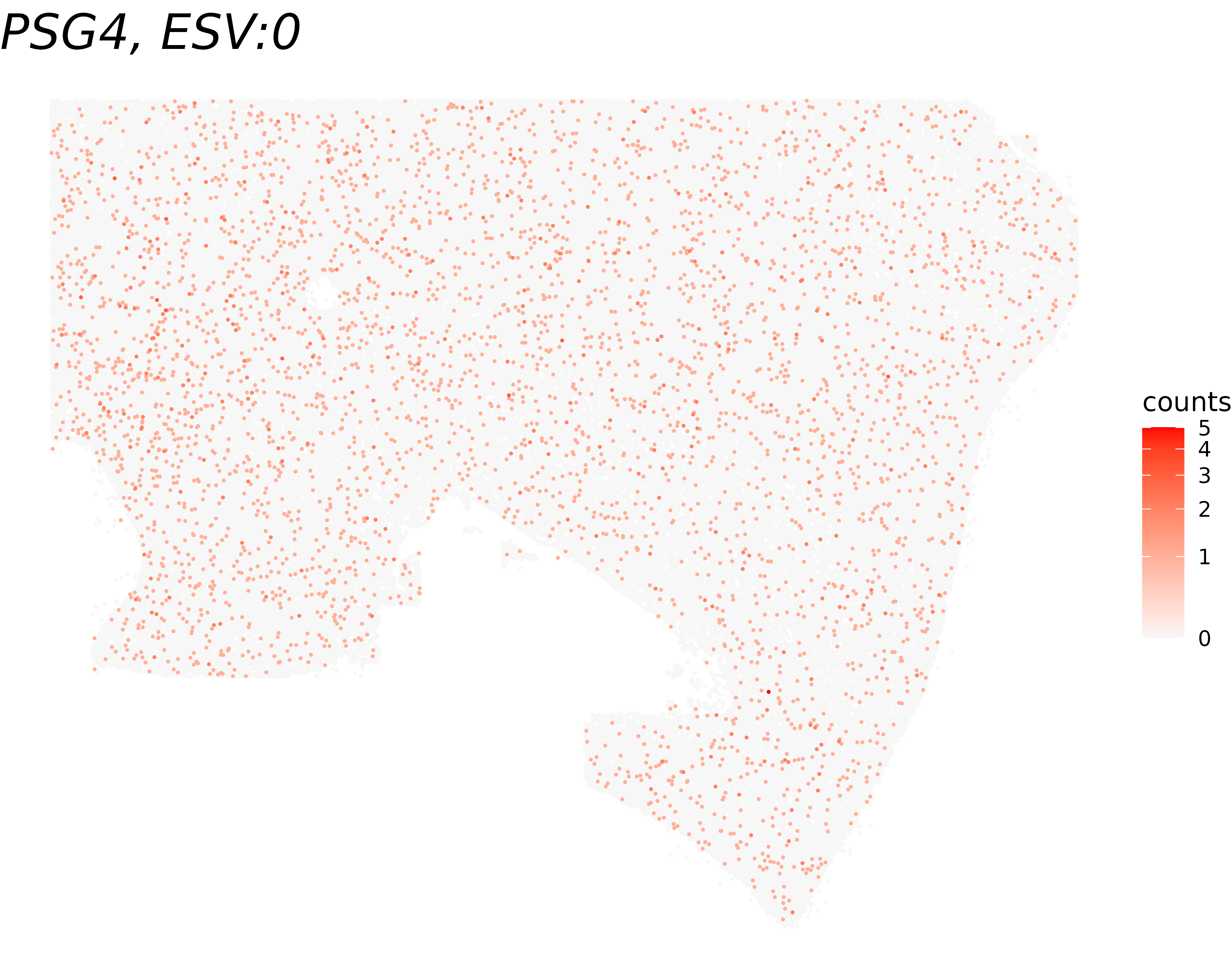
## PSG4 250.949 0.4621527 0.4621527 2.257984e-06 0.000000005. Visualize Global Spacelink Results
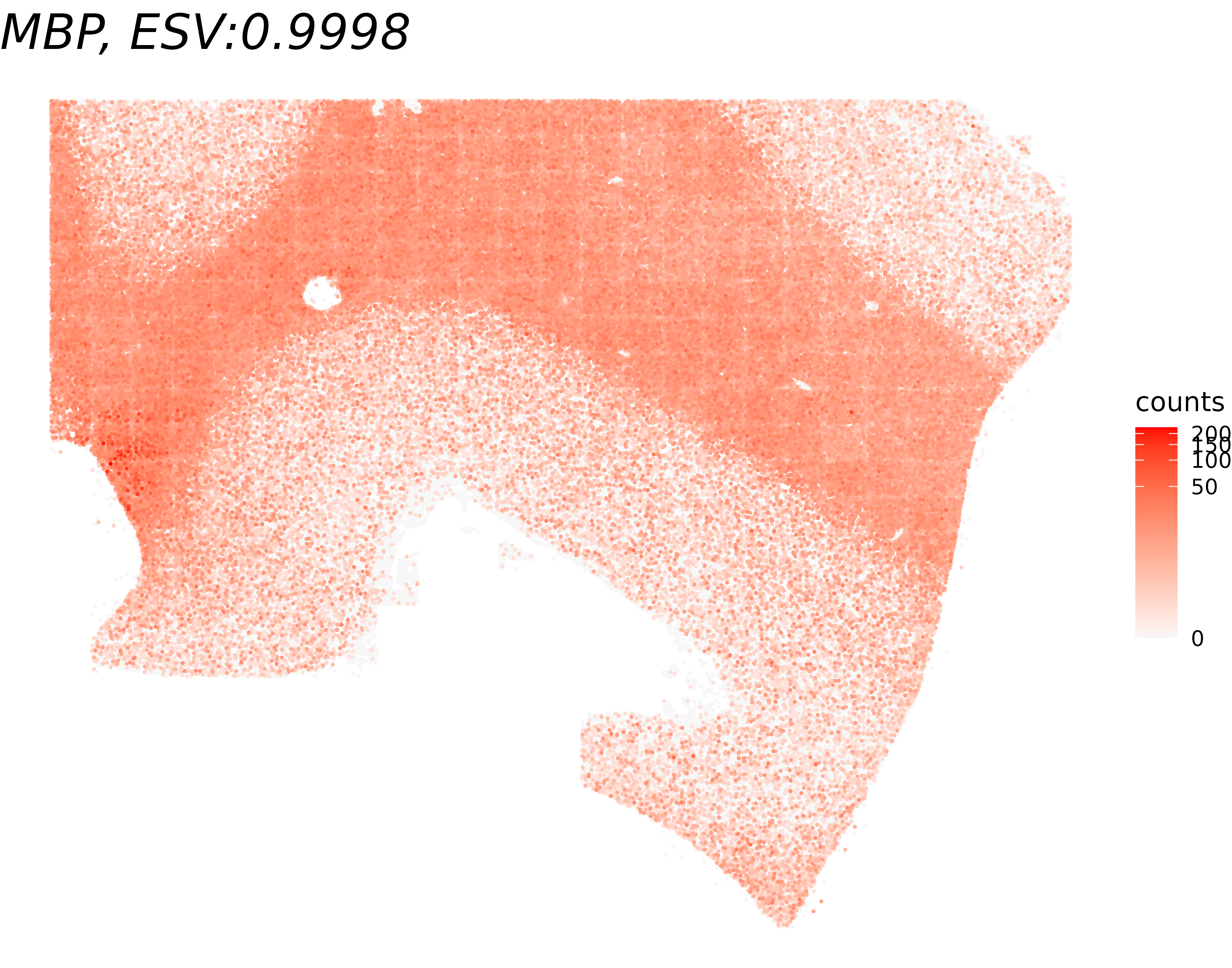
To qualitatively validate the ESV scores, we visualize gene expression for the genes with the highest and lowest ESV among the tested genes. A gene with a high ESV should display a clearly structured spatial pattern (e.g., layer-specific enrichment), while a gene with a low ESV should appear spatially random.
library(ggplot2)
library(viridis)

gene_names <- rownames(global_results)[c(which.max(global_results$ESV),
                                         which.min(global_results$ESV))]

for(gene_name in gene_names){
  df <- as.data.frame(cbind(spatial_coords, expr = counts[gene_name,]))
  colnames(df) <- c('X0', 'X1', 'expr')
  title <- paste0(gene_name, ", ESV:", round(global_results[gene_name,'ESV'],4))
  print(ggplot(df %>% arrange(expr), aes(x = X0, y = X1, color = expr)) +
    geom_point(size = 0.1) +
    ggtitle(title) + theme_void() +
    scale_color_gradient(low = "grey97", high = "red", trans = "log1p", name = "counts") +
    theme(plot.title = element_text(face = "italic", size = 20)))
}
6. Run Cell-type-specific Spacelink
Beyond global spatial variability, we may ask whether a gene’s
spatial pattern emerges specifically within a particular cell type. For
this, we use spacelink_ctSVG, which performs Spacelink
restricted to cells belonging to a specified focal cell type. When the
cell_type_proportions argument is supplied as a
binary one-hot encoded matrix (as constructed in
Section 2), the function internally detects this and subsets both the
expression matrix and spatial coordinates to cells where the focal cell
type indicator equals 1. spacelink is then applied only to
those cells, testing whether the gene is spatially variable within that
cell type’s spatial distribution.
Note that spacelink_ctSVG also supports spot-based data
with continuous cell type proportion estimates (refer to Visium
Human DLPFC Analysis).
The lite and grid_size arguments work
identically to the global spacelink() function and are
passed through to the internal call. Here we apply it to
oligodendrocytes as the focal cell type.
As before, note that padj and ESV_adj
values are computed relative to the 6 example genes only, and will
differ from a full-gene-set run.
cell_type_results <- spacelink_ctSVG(
  normalized_counts=normalized_counts[gene_list,],
  spatial_coords=spatial_coords,
  cell_type_proportions=cell_type_info,
  focal_cell_type = "oligodendrocyte",
  lite=TRUE,
  grid_size=0.1)

print(cell_type_results[order(cell_type_results$ESV_adj, decreasing=T),])
##           time         pval         padj          ESV     ESV_adj
## GFAP   138.568 0.000000e+00 0.000000e+00 1.812070e-01 0.181206965
## MBP    139.349 0.000000e+00 0.000000e+00 1.069256e-01 0.106925570
## CNP    154.706 0.000000e+00 0.000000e+00 5.807032e-02 0.058070319
## HOPX   139.915 8.518875e-72 1.277831e-71 5.427712e-03 0.005427712
## ANKRD6 148.591 5.112956e-01 5.112956e-01 1.752922e-07 0.000000000
## PSG4   140.014 2.226631e-01 2.671957e-01 2.500886e-03 0.000000000
7. Visualize Cell-type-specific Spacelink Results
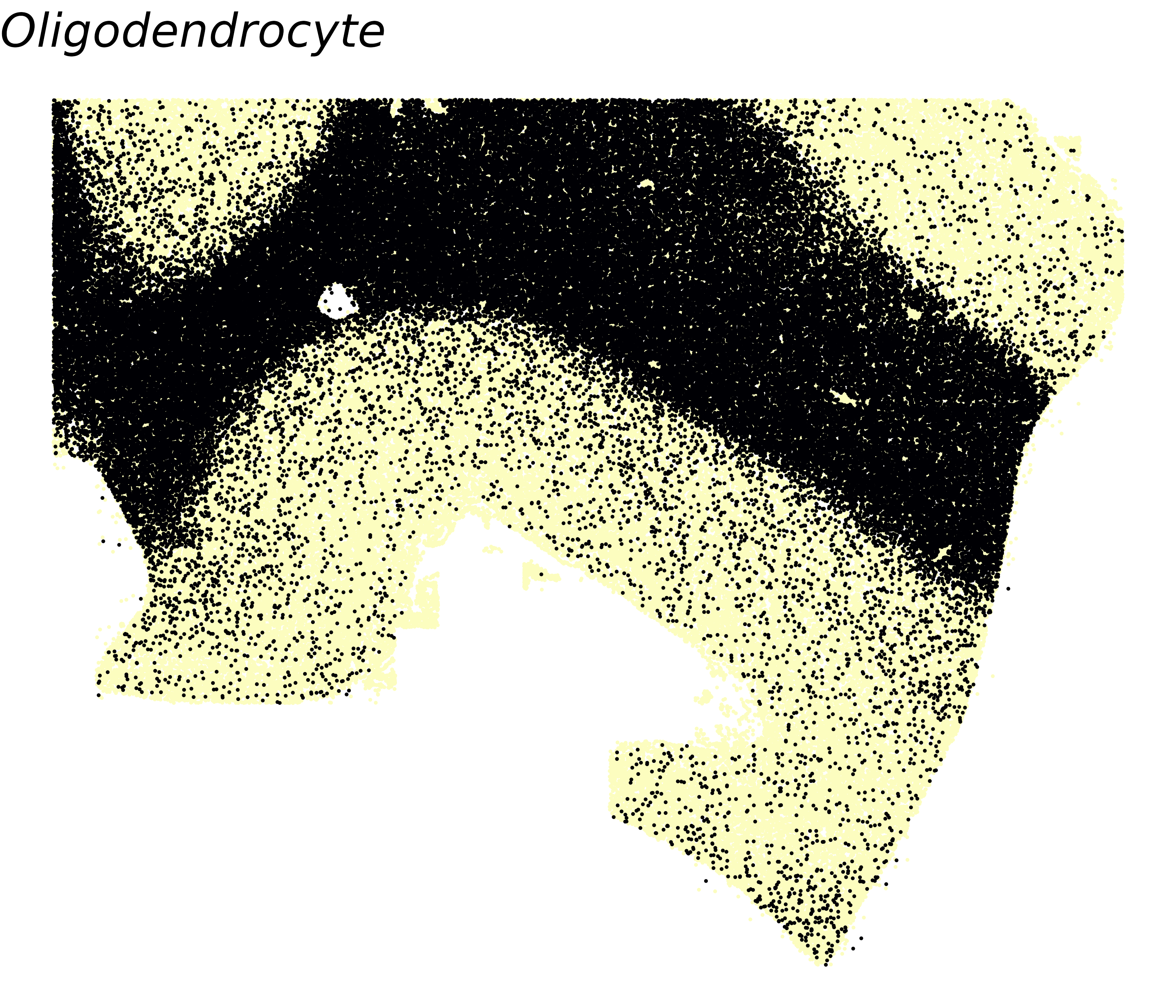
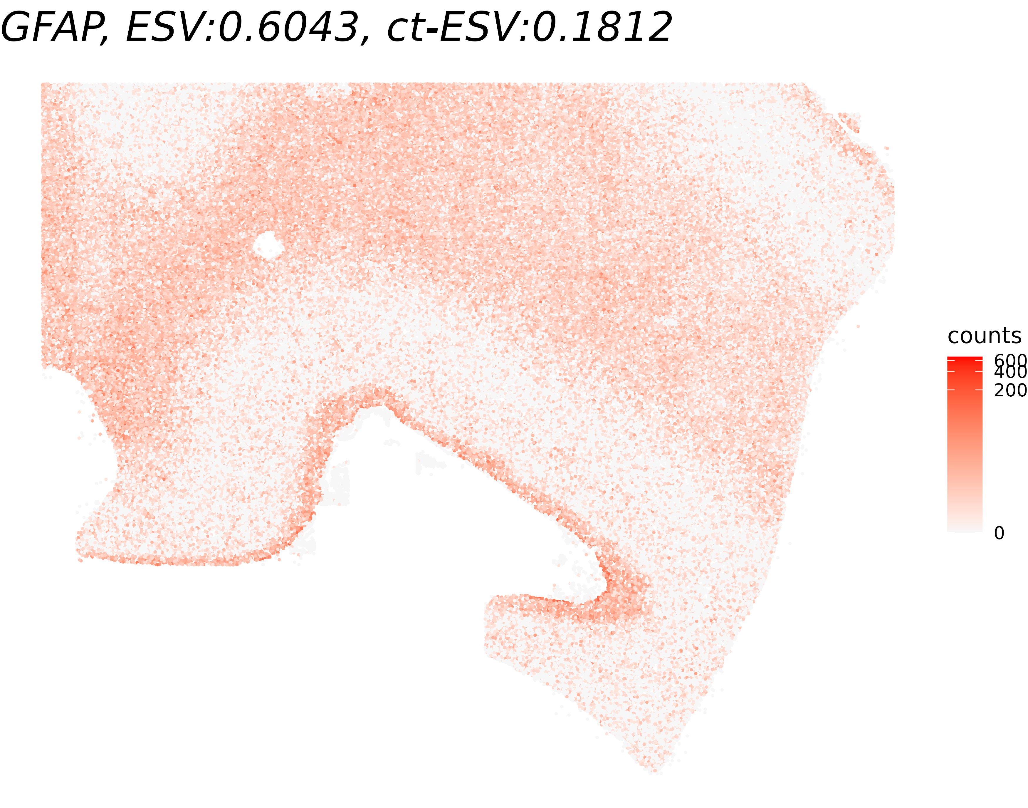
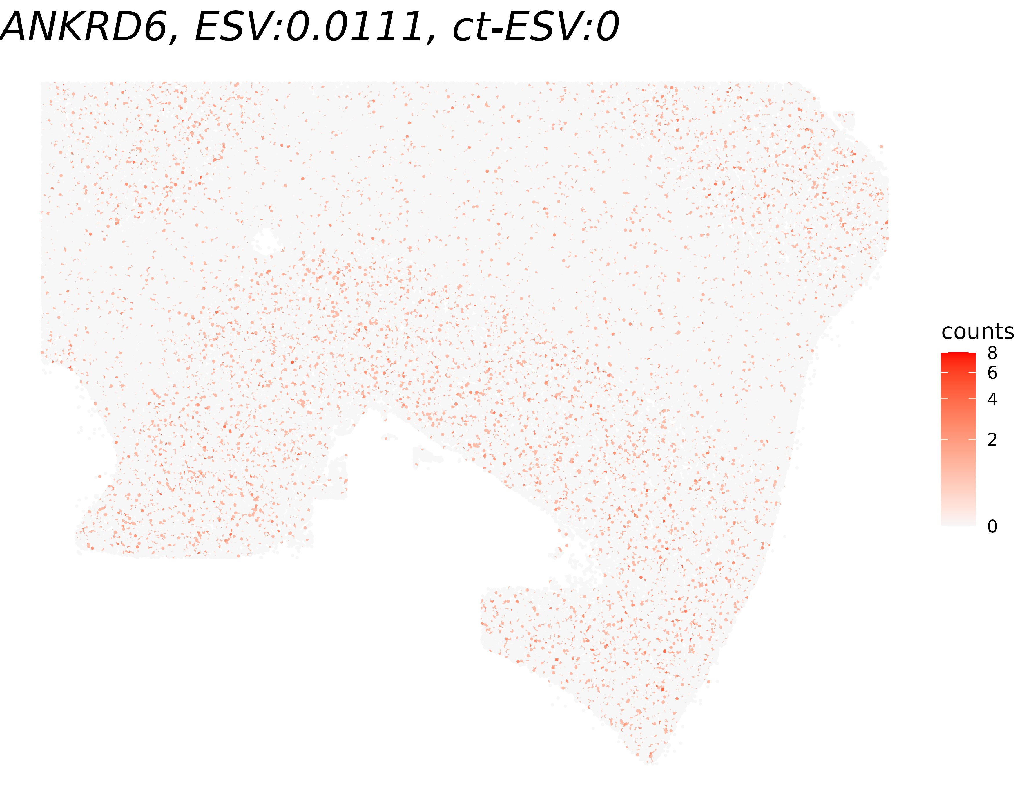
We visualize the results of cell-type-specific Spacelink to compare how a gene’s spatial pattern looks globally versus within oligodendrocytes. For each of the highest- and lowest-ct-ESV genes, we display the full spatial expression map (all cells), with the title reporting both the global ESV and the cell-type-specific ESV (ct-ESV) for reference.
We also first plot the spatial distribution of oligodendrocytes themselves. Since cell-type-specific Spacelink only tests cells of the focal type, understanding where those cells are located in the tissue helps interpret whether a gene’s ct-ESV reflects true within-type spatial variation or is driven by the cell type’s own spatial clustering.
gene_names <- rownames(cell_type_results)[c(which.max(cell_type_results$ESV_adj),
                                            which.min(cell_type_results$ESV))]

# Visualize oligodendrocyte proportions
df <- as.data.frame(cbind(spatial_coords, expr = cell_type_info[,'oligodendrocyte']))
colnames(df) <- c('X0', 'X1', 'prop')
print(ggplot(df %>% arrange(prop), aes(x = X0, y = X1, color = prop)) +
        geom_point(size = 0.1) +
        ggtitle("Oligodendrocyte") + theme_void() +
        scale_color_viridis(option="magma", direction=-1, limits=c(0,1)) +
        theme(plot.title = element_text(face = "italic", size = 20), legend.position="none"))

# Visualize gene expression (compare ESV vs ct-ESV)
for(gene_name in gene_names){
  df <- as.data.frame(cbind(spatial_coords, expr = counts[gene_name,]))
  colnames(df) <- c('X0', 'X1', 'expr')
  title <- paste0(gene_name,
                ", ESV:", round(global_results[gene_name,'ESV'],4),
                ", ct-ESV:", round(cell_type_results[gene_name,'ESV'],4))
  print(ggplot(df, aes(x = X0, y = X1, color = expr)) +
        geom_point(size = 0.1) +
        ggtitle(title) + theme_void() +
        scale_color_gradient(low = "grey97", high = "red", trans = "log1p", name = "counts") +
        theme(plot.title = element_text(face = "italic", size = 20)))
}