Visium Human DLPFC Analysis • spacelink

Application of Spacelink to Visium Human DLPFC Dataset

Here, we demonstrate how to perform SVG analysis using the spacelink package with a Visium human dorsolateral prefrontal cortex (DLPFC) dataset. The dataset is available here, and we use sample 151673. Cell-type proportions were estimated using RCTD with the CosMx Human Frontal Cortex dataset as a reference. The processed example data, provided as Visium_human_DLPFC, includes gene expression, spot coordinates, and the estimated cell type proportions.

We walk through the full Spacelink workflow in two stages: (1) global tissue-level SVG detection, which tests for spatial variability across all spots regardless of cell type, and (2) cell-type-specific SVG detection, which tests for spatial variability within a specific cell population.

1. Load Packages

library(spacelink)
library(Seurat)
library(sctransform)
library(ggplot2)
library(viridis)

2. Load Example Dataset

Here we load the built-in example dataset for Visium Human DLPFC (sample 151673). It comes with three pieces of information we’ll use throughout the analysis:

counts: Gene expression matrix (33,538 genes × 3,639 spots)
spatial_coords: Spatial coordinates for each spot
cell_type_proportions: Estimated cell type compositions via RCTD (9 cell types)

data(Visium_human_DLPFC)
counts <- Visium_human_DLPFC$counts
spatial_coords <- Visium_human_DLPFC$spatial_coords
cell_type_proportions <- Visium_human_DLPFC$cell_type_proportions
head(counts[,1:10])

## 6 x 10 sparse Matrix of class "dgTMatrix"
##   [[ suppressing 10 column names ‘AAACAAGTATCTCCCA-1’, ‘AAACAATCTACTAGCA-1’, ‘AAACACCAATAACTGC-1’ ... ]]                               
## MIR1302-2HG . . . . . . . . . .
## FAM138A     . . . . . . . . . .
## OR4F5       . . . . . . . . . .
## AL627309.1  . . . . . . . . . .
## AL627309.3  . . . . . . . . . .
## AL627309.2  . . . . . . . . . .

head(spatial_coords)

##                    pxl_col_in_fullres pxl_row_in_fullres
## AAACAAGTATCTCCCA-1               9791               8468
## AAACAATCTACTAGCA-1               5769               2807
## AAACACCAATAACTGC-1               4068               9505
## AAACAGAGCGACTCCT-1               9271               4151
## AAACAGCTTTCAGAAG-1               3393               7583
## AAACAGGGTCTATATT-1               3665               8064

head(cell_type_proportions)

##                     endothelial       L2_3           L4           L6 oligodendrocyte          OPC       astro         Inh    microglia
## AAACAAGTATCTCCCA-1 2.331552e-02 0.86383709 9.941496e-05 8.994572e-05     0.008841064 8.994572e-05 0.037094727 0.060440671 0.0061916188
## AAACAATCTACTAGCA-1 7.952809e-02 0.55623941 1.284478e-04 1.413909e-02     0.001048564 1.284478e-04 0.083634323 0.264896732 0.0002568957
## AAACACCAATAACTGC-1 4.144100e-05 0.07909515 4.144100e-05 8.593492e-02     0.826629114 7.799136e-05 0.006276291 0.000124323 0.0017793364
## AAACAGAGCGACTCCT-1 4.419690e-04 0.70660998 1.437067e-04 1.437067e-04     0.012711896 1.437067e-04 0.119882025 0.133047245 0.0268757663
## AAACAGCTTTCAGAAG-1 1.398113e-02 0.52170271 8.882893e-05 2.874930e-01     0.050319200 8.882893e-05 0.026019353 0.096453571 0.0038533732
## AAACAGGGTCTATATT-1 8.872097e-05 0.37248441 8.872097e-05 3.500929e-01     0.206785555 8.872097e-05 0.029330741 0.040862758 0.0001774419

3. Preprocessing

Before running the analysis, we do a bit of cleaning. First, we remove mitochondrial genes since high mitochondrial expression usually signals low-quality or damaged cells rather than real biology. We also drop genes that are expressed in very few spots (less than 0.5%), as they don’t carry enough information to be useful. Finally, we normalize the counts using SCTransform, which corrects for differences in sequencing depth across spots.

counts <- counts[!grepl("(^MT-)|(^mt-)", rownames(counts)),]
counts <- counts[apply(counts >= 3, 1, sum) >= ncol(counts)*0.005,]
dim(counts)

## [1] 3309  3639

seurat_obj <- CreateSeuratObject(counts = counts)
seurat_norm = SCTransform(seurat_obj, vst.flavor = "v2", verbose = FALSE)
normalized_counts <- seurat_norm@assays$SCT$data
head(normalized_counts[,1:10])

## 6 x 10 sparse Matrix of class "dgCMatrix"
##   [[ suppressing 10 column names ‘AAACAAGTATCTCCCA-1’, ‘AAACAATCTACTAGCA-1’, ‘AAACACCAATAACTGC-1’ ... ]]                                                    ##                             
## HES4  0.6931472 .        . .         .         .         . .         .         .
## ISG15 .         .        . .         0.6931472 .         . 0.6931472 .         .
## AGRN  0.6931472 1.386294 . .         0.6931472 .         . 0.6931472 .         .
## SDF4  0.6931472 .        . 0.6931472 .         .         . .         0.6931472 .
## ACAP3 0.6931472 .        . .         .         .         . .         0.6931472 .
## DVL1  .         .        . .         .         0.6931472 . .         .         .

4. Run Global Spacelink

Now we’re ready to run the main analysis. Here we use spacelink to identify spatially variable genes (SVGs) across the tissue. We’ll test this on 6 example genes to keep things simple. The two numbers to pay attention to in the results are padj (whether the spatial autocorrelation is statistically significant) and ESV_adj (how strong that spatial autocorrelation is, on a scale from 0 to 1). Note that the padj and ESV_adj values will differ when running the analysis on the full gene set, because the Benjamini–Hochberg adjustment is applied across all genes. In this example, the adjustment is performed using only the six selected genes.

gene_list <- c("CNP","EIF5B","HOPX","KRT19","PHB","SHISA5")
global_results <- spacelink(
  normalized_counts = normalized_counts[gene_list,],
  spatial_coords = spatial_coords
)
print(global_results[order(global_results$ESV_adj, decreasing=T),c("time","pval","padj","ESV","ESV_adj")])

##         time       pval        padj         ESV     ESV_adj
## CNP    4.082 0.00000000 0.000000000 0.982947579 0.982947579
## HOPX   3.904 0.00000000 0.000000000 0.709631417 0.709631417
## KRT19  3.792 0.00000000 0.000000000 0.684495108 0.684495108
## EIF5B  3.736 0.00373013 0.005595195 0.025783391 0.025783391
## SHISA5 3.736 0.02000210 0.024002518 0.009663969 0.009663969
## PHB    3.734 0.10824339 0.108243395 0.026795125 0.000000000

5. Visualize Global Spacelink Results

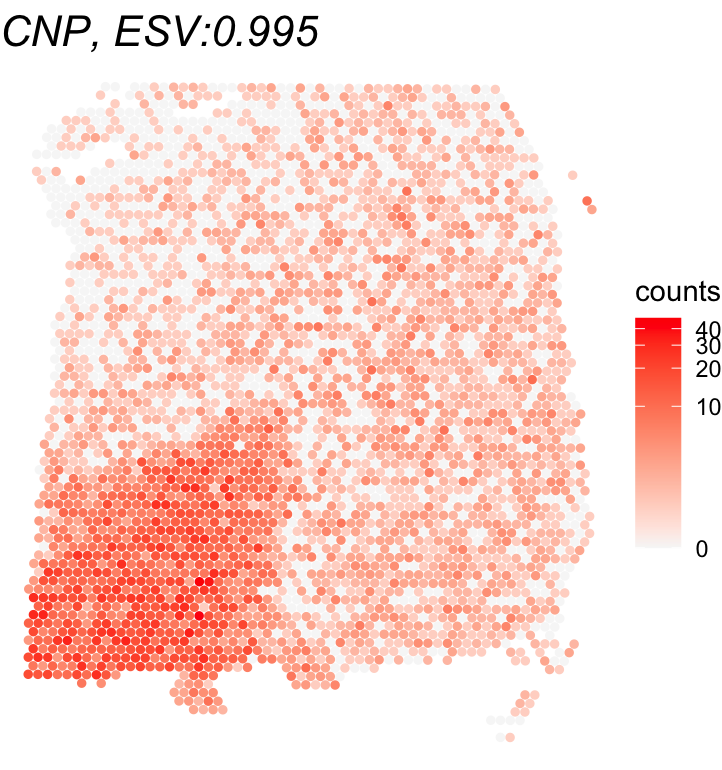
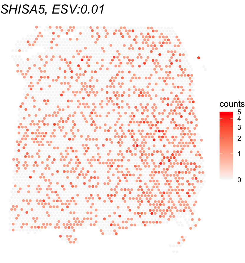
To get an intuitive sense of what the ESV score means, let’s plot the gene with the highest ESV alongside the one with the lowest. This gives us a side-by-side comparison of a strong SVG vs. a non-SVG, showing how differently their expression is distributed across the tissue.

gene_names <- rownames(global_results)[c(which.max(global_results$ESV_adj),
                                         which.min(global_results$ESV))]

for(gene_name in gene_names){
  df <- as.data.frame(cbind(spatial_coords, expr = counts[gene_name,]))
  colnames(df) <- c('X0', 'X1', 'expr')
  title <- paste0(gene_name, ", ESV:", round(global_results[gene_name,'ESV'],3))
  print(ggplot(df, aes(x = X0, y = X1, color = expr)) +
    geom_point(size = 1) +
    ggtitle(title) + theme_void() + scale_y_reverse() +
    scale_color_gradient(low = "grey97", high = "red", trans = "log1p", name = "counts") +
    theme(plot.title = element_text(face = "italic", size = 16)))
}

6. Run Cell-type-specific Spacelink

Here, we dig a little deeper by asking whether a gene’s spatial pattern emerges within a particular cell type. We use spacelink_ctSVG with oligodendrocyte as our focal cell type. The ct-ESV score in the output works the same way as ESV, but specifically reflects variability tied to that cell type. Again, note that the padj and ESV_adj values will differ when running the analysis on the full gene set, because the Benjamini–Hochberg adjustment is applied across all genes. In this example, the adjustment is performed using only the six selected genes.

cell_type_results <- spacelink_ctSVG(
  normalized_counts = normalized_counts[gene_list,],
  spatial_coords = spatial_coords,
  cell_type_proportions = cell_type_proportions,
  focal_cell_type = "oligodendrocyte"
)

print(cell_type_results[order(cell_type_results$ESV_adj, decreasing=T),])

##           time         pval         padj          ESV   ESV_adj
## KRT19  112.470 2.295822e-06 6.887466e-06 7.762241e-01 0.7762241
## CNP    130.494 7.442970e-07 4.465782e-06 6.518893e-01 0.6518893
## EIF5B  148.584 2.066347e-01 4.132695e-01 2.195354e-01 0.0000000
## HOPX   121.434 9.434479e-01 9.434479e-01 2.236363e-05 0.0000000
## PHB    144.309 3.258193e-01 4.887289e-01 4.234864e-02 0.0000000
## SHISA5 149.888 6.209340e-01 7.451208e-01 1.455330e-02 0.0000000

7. Visualize Cell-type-specific Spacelink Results

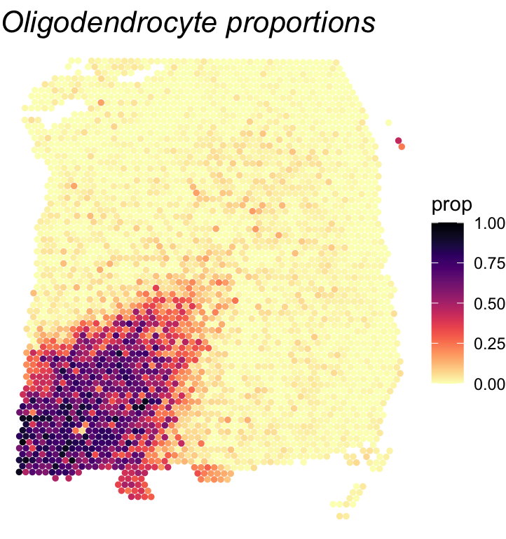
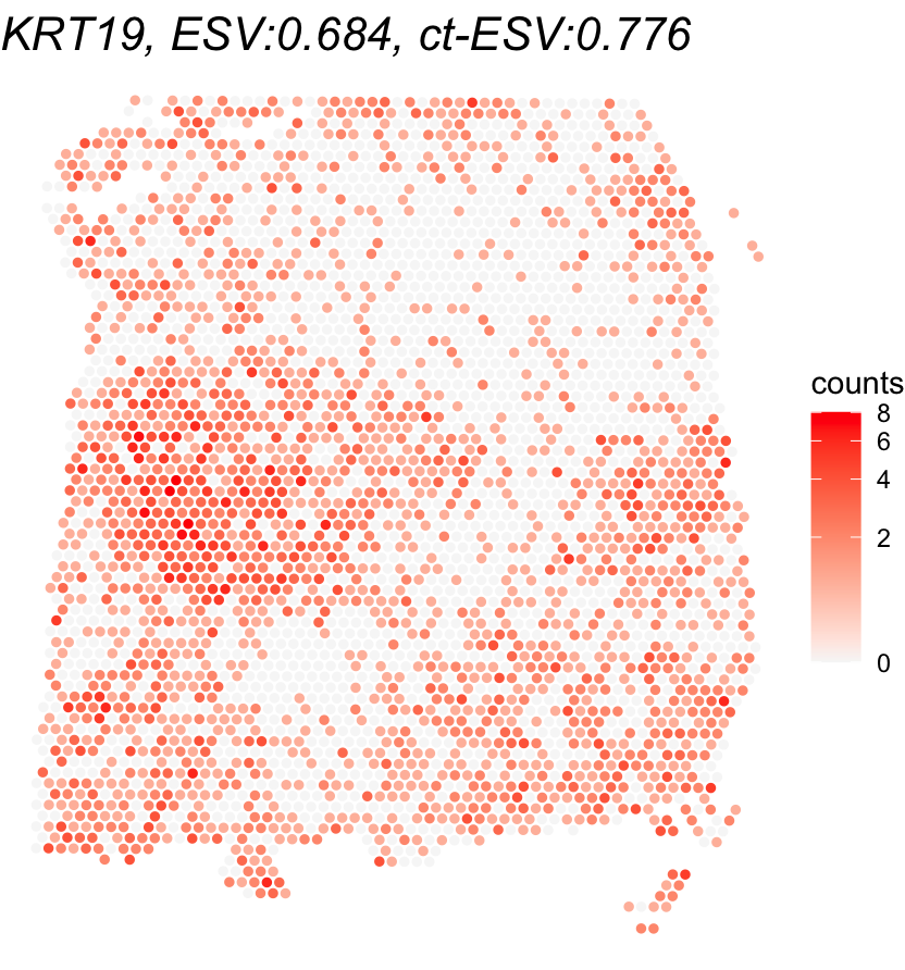
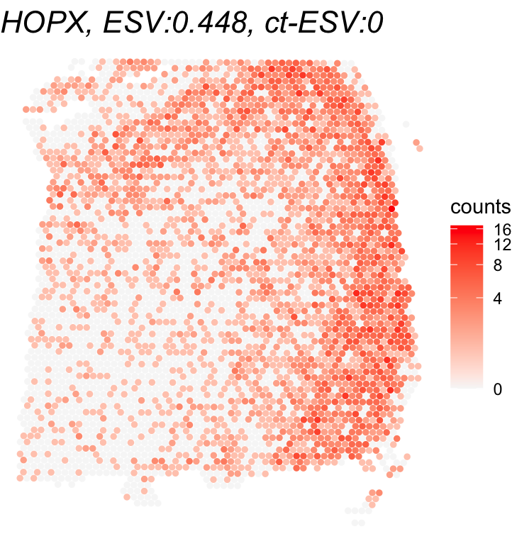
To wrap up, we visualize the results of the cell-type-specific analysis. We first plot the oligodendrocyte proportions across the tissue to see where this cell type is concentrated. Then, we compare the gene with the highest ct-ESV to the one with the lowest. Looking at both ESV and ct-ESV together helps us understand whether a gene’s spatial pattern is really being driven by oligodendrocytes or by something else entirely.

gene_names <- rownames(cell_type_results)[c(which.max(cell_type_results$ESV_adj),
                                            which.min(cell_type_results$ESV))]

# Visualize oligodendrocyte proportions
df <- as.data.frame(cbind(spatial_coords, expr = cell_type_proportions[,'oligodendrocyte']))
colnames(df) <- c('X0', 'X1', 'prop')
print(ggplot(df, aes(x = X0, y = X1, color = prop)) +
        geom_point(size = 1) +
        ggtitle("Oligodendrocyte proportions") + theme_void() + scale_y_reverse() +
        scale_color_viridis(option="magma", direction=-1, limits=c(0,1)) +
        theme(plot.title = element_text(face = "italic", size = 16)))

# Visualize gene expression (compare ESV vs ct-ESV)
for(gene_name in gene_names){
  df <- as.data.frame(cbind(spatial_coords, expr = counts[gene_name,]))
  colnames(df) <- c('X0', 'X1', 'expr')
  title <- paste0(gene_name,
                  ", ESV:", round(global_results[gene_name,'ESV'],3),
                  ", ct-ESV:", round(cell_type_results[gene_name,'ESV'],3))
  print(ggplot(df, aes(x = X0, y = X1, color = expr)) +
          geom_point(size = 1) +
          ggtitle(title) + theme_void() + scale_y_reverse() +
          scale_color_gradient(low = "grey97", high = "red", trans = "log1p", name = "counts") +
          theme(plot.title = element_text(face = "italic", size = 16)))
}